
General Information
Subject Area: Mathematics (B.E.S.T.)
Grade: 912
Strand: Data Analysis and Probability
Date Adopted or Revised: 08/20
Status: State Board Approved
Benchmark Instructional Guide
Connecting Benchmarks/Horizontal Alignment
Terms from the K-12 Glossary
- Line of Fit
- Numerical Data
- Scatter Plot
Vertical Alignment
Previous Benchmarks
Next Benchmarks
Purpose and Instructional Strategies
In grade 8, students informally fitted a line to a scatter plot. In Algebra I, students look more closely at lines of fit and assess their quality by looking at the signs and sizes of the residuals. In later courses, students will use the residuals to determine the correlation coefficient to assess the quality of fit.- For students to have a full understanding of the quality of a line of fit, this benchmark should be combined with MA.912.DP.2.4 and MA.912.DP.2.6.
- Instruction includes matching scatter plots with residual plots, matching residuals for strength/direction and considering the residual data points themselves.
- Instruction focuses on real-world contexts and includes the use of technology.
- A residual plot has the residual values on the vertical axis; the horizontal axis displays the -variable.
- A residual value is a measure of how far a data value is from the estimate calculated from the line of fit.
- Residuals are positive if data points are above the line of fit and negative if data points are below the line of fit. When creating a residual plot, students should understand that residuals with a positive -value represent a data point that was above the line of fit (a value that was more than the model predicted). Residuals with a negative -value represents a data point that was below the line of fit (a value that was less than the model predicted).
- To calculate the residual, students use the line of fit and take the difference between an input’s actual value and its predicted value (MTR.3.1). This can correspond to the equation = −, where represents the residual, represents the -coordinate of data value and represents the -coordinate of predicted value.
- Once residuals are calculated, students can determine the number of positive and negative residuals and the largest and smallest residuals.
- Outliers, which are observed data points that are far from a line of fit, can be determined from the residual as points whose residuals have a large absolute value.
- To assess the fit of a given linear function the residual plot will show points randomly scattered around the center line of zero (-axis), with no obvious, non-random pattern (MTR.5.1).
- If the residual plot shows a pattern, such as a u-shaped pattern, that indicates that a nonlinear model would be a better fit for the data.
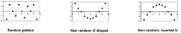
- If the residual plot shows a pattern, such as a u-shaped pattern, that indicates that a nonlinear model would be a better fit for the data.
Common Misconceptions or Errors
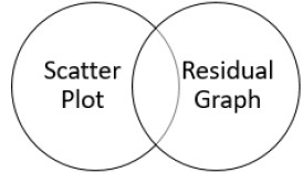
- Students may not be able to distinguish between a scatter plot and a residual graph.
- Students may have difficulty finding the residual value if the actual -value equals the predicted -value.
- Students may forget that residual graphs consist of the ordered pair (-value, residual).
- Students may not be able to determine an appropriate model (linear/nonlinear) from a residual graph.
Strategies to Support Tiered Instruction
- Instruction includes vocabulary development by co-creating a graphic organizer for scatter plot and residual graph.
- Teacher co-creates an anchor chart that provides examples of residual graphs for linear models.
- Instruction includes the opportunity to use colors to identify the - and -values in the original data and the - and -values in the ordered pairs associated with the residual graph, and highlight the - and -axis of the residual graph in the same color in order to see the relationship.
- For example, for the data point (6, −0.5), the residual point is (6, −0.85) based on the line fit being = −0.6 + 2.25.
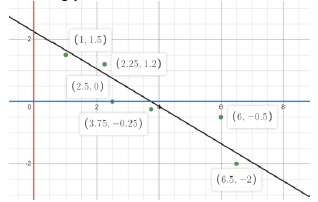
- For example, for the data point (6, −0.5), the residual point is (6, −0.85) based on the line fit being = −0.6 + 2.25.
Instructional Tasks
Instructional Task 1 (MTR.4.1, MTR.5.1, MTR.7.1)- Crickets are one of nature’s more interesting insects, partly because of their musical ability. In England, the chirping or singing of a cricket was once considered to be a sign of good luck. Crickets will not chirp if the temperature is below 40 degrees Fahrenheit (°F) or above 100 degrees Fahrenheit (°F). A table is given with some data collected.
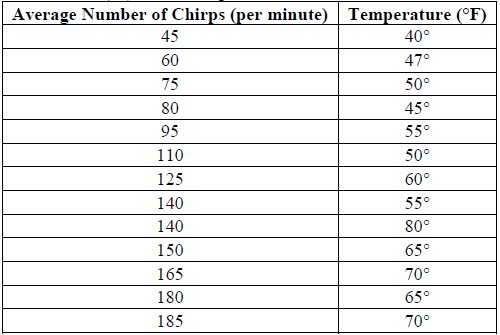
- Part A. Based on the data, the line of best fit can be described by the model = 0.214 + 32.317. Create a residual plot using technology.
- Part B. What do you notice about the positive and negative residuals?
- Part C. If the number of chirps is 45, what temperature is predicted by the line of best fit? How does this compare with the data?
- Part D. Write an equation that compares the residual, the predicted value and the data value.
- Part E. What are the largest and the smallest residuals?
- Part F. Based on the residual plot, can you determine if there are any possible outliers in the data?
- Part G. Does the residual plot indicate that a linear model is appropriate for this data?
Instructional Items
Instructional Item 1- Based on the data, we know using technology that the line of best fit for the relationship between grams of fat and the total calories in fast food using the given data below can be represented by = 11.44 + 219.89.
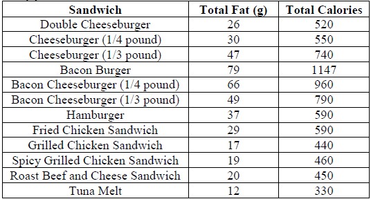
- Part A. Calculate the residuals and plot them on a residual plot where grams of fat are the -variable.
- Part B. Which sandwiches have the residuals with the largest and smallest absolute values?
- Part C. Is a linear model reasonable for this data set?
*The strategies, tasks and items included in the B1G-M are examples and should not be considered comprehensive.